

not logged in | [Login]
![]()
This module calculates the energy supply potential and related costs for rooftop installed solar thermal and PV systems in a defined area. The inputs to the module are raster files of building footprint and solar irradiation, costs and efficiency of reference solar thermal and PV systems and the fractions of usable rooftop area where solar thermal and PV systems are installed.
The calculation module aims to compute the solar thermal and the photovoltaic energy potential and the financial feasibility of a selected area by considering:
The input parameters and layers, as well as output layers and parameters, are as follows.
Input layers and parameters are:
Output layers and parameters are:
Starting from the available area and the kind of PV technology the module computes the PV energy production under the following assumptions:
These assumptions have been done in order to consider a planning phase for a region and not the design of a specific PV system.
The yearly energy output is derived by considering the spatial distribution of yearly solar radiation on the building footprint. The PV energy production is computed for a single representative plant. The most representative installed peak power for a PV system is an input of the module. Consequently, the surface covered by a single plant and the total number of plants are computed.
Finally, the most suitable area is computed by considering the roofs with higher energy production. The energy production of each pixel considers covering only a fraction of the roofs equal to f_roof. The integral of the energy production of the most suitable area is equal to the total energy production of the selected area.
To give a practical example, the CM logic/methodology is applied to a predefined area. By default, the input area we are using is the buildings' footprint. So for example, the city of Bolzano (Italy), since a large part of the city is the historic centre (where it is not possible to install solar panels) we can estimate that only 1 roof every 5 can be used to collect solar energy (~20%). Instead, if you provide an area that it is available to implement some solar field then you can set 100% of the area can be used for the solar system.
Which area of the 20% of the roofs in Bolzano can be covered by PV panels? Cover the whole roof is not realistic, since part of the roof have not suitable orientation. Since the building generally has 4 sides, we can imagine that around 25% of the roof have a good orientation (at least in Bolzano, where most of the roofs are not plane and have 2 or 4 roofs slopes). Nevertheless, we have shadowing effects from the surrounding trees, buildings, mountains, etc, and generally, we are leaving some space close to the border of the roofs so let's imagine that 50% of the good oriented roof can be used by PV (25% * 50% = 12.5%), the default value is a bit more optimistic (15%).
In case of a solar field generally, the PV string occupies around 40-50% of the area to avoid the shadowing effect between PV strings.
For the sake of example, we are explaining the methodology for one single pixel (1 hectare area). The CM applies the same logic for each pixel in the area selected by the user. The default layer (the building footprint) has a pixel dimension of 100x100m, therefore we have an available surface of 10000 m². For this example imagine that only 3000 m² of roofs are available in the pixel, the other missing part of the surface is surface dedicated to routes, green areas, river, etc. The logic implemented by the CM is:
available_surface = 3000 [m²] * 20% = 600 [m²]
available_pv_surface = 600 [m²] * 12.5% = 75 [m²]
single_pv_surface = 3 [kWp] / 0.15 = 20 [m²]
n_pv_plants = 75 [m²] // 20 [m²] = 3
and therefore we will have 3 plants of 3 KWp installed on the pixel of 100 by 100 m (so 9 kWp), and then we multiply this value by the energy produced by 1 kWp and multiply by the efficiency of the PV systems (inverter and transmission, by default: 0.85) to obtain the total energy produced by the pixel:
pv_energy = solar_radiation [kWh/kWp/year] * 9 [kWp] * 0.85
Now we have a pixel of 100x100m that it is available for a PV field system:
available_surface = (100 x 100) [m²] * 100% = 10000 [m²]
available_pv_surface = 10000 m² * 50% = 5000 m²
single_pv_surface = 3 [kWp] / 0.15 = 20 [m²]
n_pv_plants = 5000 // 20 = 250
and therefore we will have 250 plants of 3 KWp installed on the pixel of 100 by 100 m (so 750 kWp), and then we multiply this value by the hourly energy produced by 1 kWp and multiply by the efficiency of the PV systems (inverter and transmission, by default: 0.85) to obtain the total energy produced by the pixel:
pv_energy = solar_radiation [kWh/kWp/year] * 750 kWp * 0.85
The building surface that can be used, is a limited resource. Therefore it is not possible to use the same surface to collect solar energy with a PV system and at the same time, use a Solar Thermal system. So recalling the previous example, we have already 75 m² of surface dedicated to PV, we estimated that the good-oriented roof accounts for 25% of the total surface and therefore, we have still other 75 [m²] available. We can only use a fraction, let's say that 7.5%. This means that if before we consider a 25% of the roof with a good exposition then we are considering the 12.5% is dedicated to the PV and 7.5 is dedicated to ST, and therefore, we are using 20% of the 25%.
So to give a practical example:
available_surface = 3000 [m²] * 20% = 600 [m²]
available_st_surface = 600 [m²] * 7.5% = 45 [m²]
note that 75 + 45 = 120 [m²] that it is smaller than the estimated surface that could have a good exposition (available_surface * 25% = 150 [m²]).n_st_plants = 45 [m²] // 5 [m²] = 9
solar_radiation [kWh/m²] * 45 [m²] * 0.85
Here you get the bleeding-edge development for this calculation module.
Here, the calculation module is run for the Lombardy region in Italy (NUTS2).
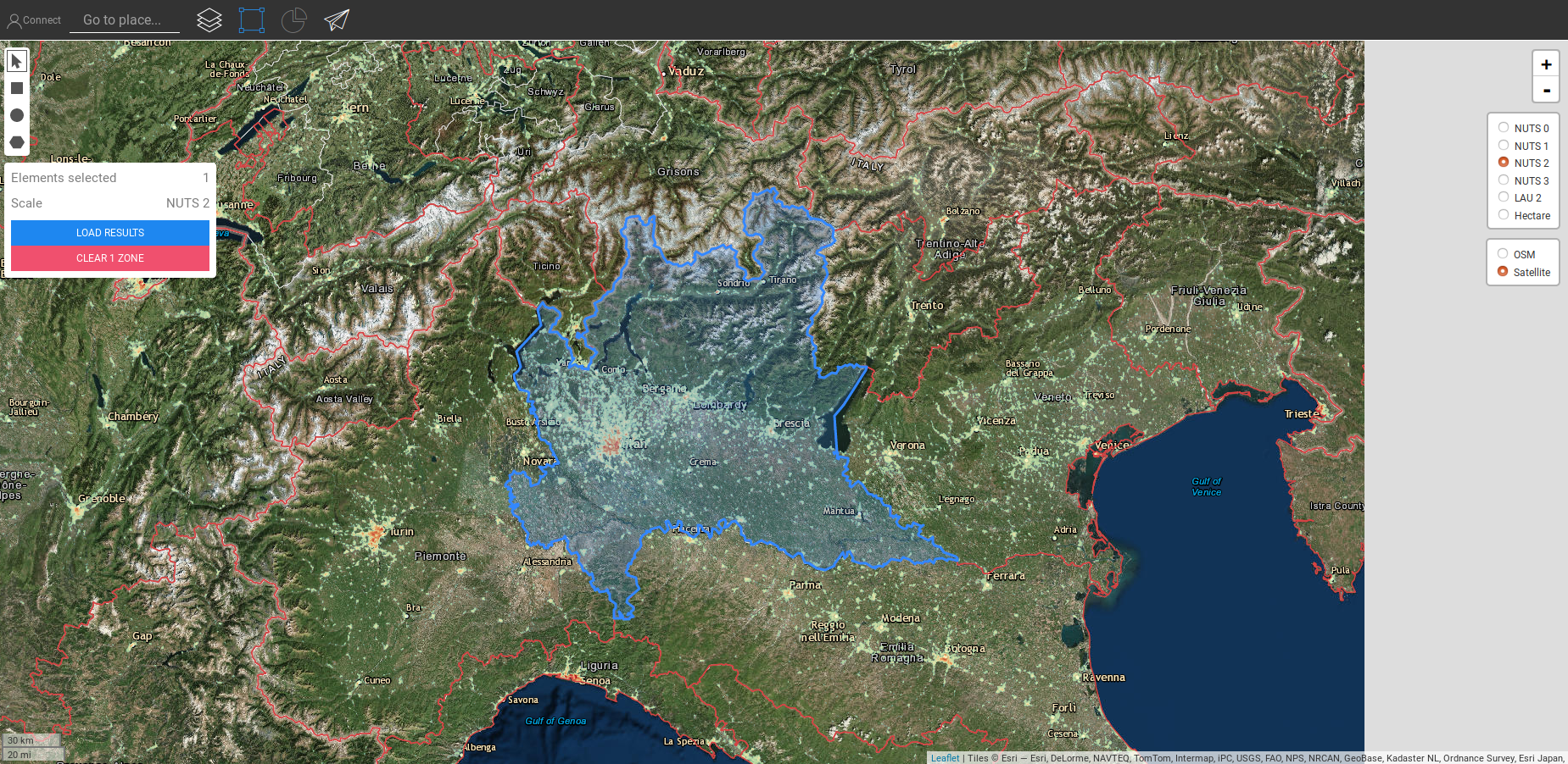 Fig. 1: Select a region
Follow the steps as shown in the figure below:
Now, the "Solar PV Potential" opens and is ready to run.
The default input values consider the possibility to install roof-mounted PV panels on buildings. These values refer to a plant of 3 kWp. You may need to set values bellow or above default values considering additional local considerations and costs. Therefore, the user should tweak these values to find the best combination of thresholds for his/her case study.
To run the calculation module, follow the next steps:


Depending on your experience and local knowledge, you may increase or decrease the input values to obtain better results. You may decide to increase the building surface suitable for PV plants.
Assign a name to the run session (optional - here, we chose "Test Run 2") and set the input parameters Percentage of buildings with solar panels equal to 50. It means that we are covering 50% of the available building roofs. Notice that since each pixel can represent more than one building and we are not covering the whole roof with PV panels, the user can set also the Effective building roof utilization factor. The default value is set to 0.15. This means that only 15% of the roof surface in a pixel is covered by PV panels.
Wait until the process is finished.
Giulia Garegnani, in Hotmaps-Wiki, CM-Solar-PV-potential (April 2019)
This page was written by Giulia Garegnani (EURAC).
☑ This page was reviewed by Mostafa Fallahnejad (EEG - TU Wien).
Copyright © 2016-2020: Giulia Garegnani
Creative Commons Attribution 4.0 International License
This work is licensed under a Creative Commons CC BY 4.0 International License.
SPDX-License-Identifier: CC-BY-4.0
License-Text: https://spdx.org/licenses/CC-BY-4.0.html
We would like to convey our deepest appreciation to the Horizon 2020 Hotmaps Project (Grant Agreement number 723677), which provided the funding to carry out the present investigation.
View in another language:
Bulgarian* Czech* Danish* German* Greek* Spanish* Estonian* Finnish* French* Irish* Croatian* Hungarian* Italian* Lithuanian* Latvian* Maltese* Dutch* Polish* Portuguese (Portugal, Brazil)* Romanian* Slovak* Slovenian* Swedish*
* machine translated